30 September 2026 · 7 min read
Batch vs stochastic vs mini-batch gradient descent, and how to choose a batch size
Batch, stochastic, and mini-batch gradient descent differ only in how many training examples each update looks at. This post explains what that changes, why mini-batch is the usual choice, and how to pick a batch size and adjust the learning rate with it.
Batch, stochastic, and mini-batch gradient descent are three versions of the same training procedure that differ in how many training examples the model looks at before each weight update. Batch gradient descent uses the whole dataset, stochastic gradient descent uses one example, and mini-batch gradient descent uses a small random group, usually 32 to 512 examples. That number is the batch size, and it decides how long each step takes, how noisy it is, how much memory it needs, and which learning rate works.
The update rule all three share
Training adjusts a model's parameters, written $\theta$, to make a loss $L$ smaller. The loss is one number that scores how wrong the model's predictions are. Its gradient, $\nabla L$, holds one number per parameter saying which way and how steeply the loss rises when that parameter grows. Gradient descent moves each parameter a small step the other way, scaled by the learning rate $\eta$:
$$\theta \leftarrow \theta - \eta \cdot \nabla L$$
The loss is an average over a set of training examples, so the gradient is an average too, and the three variants differ in which set they average over. The gradient descent post covers the rule itself in more depth.
Batches and epochs
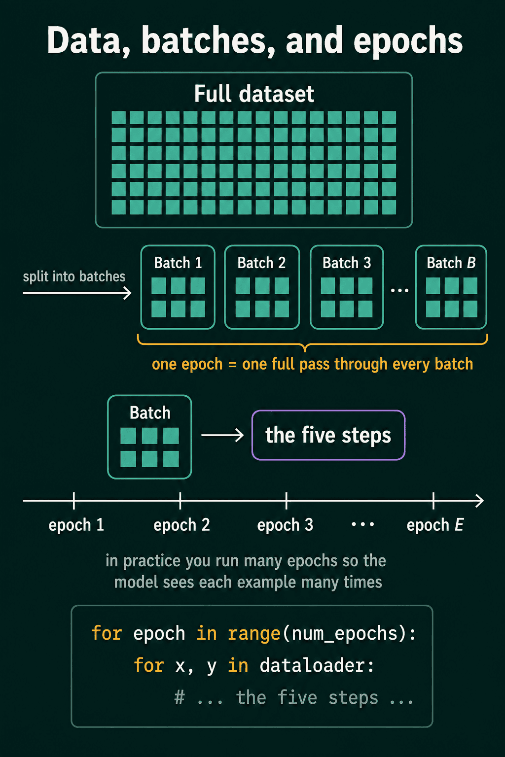
In code, the training data is split into batches, and each batch goes through one training step: the model predicts, the loss is computed, the old gradients are cleared, backpropagation computes new gradients, and the optimizer updates the weights. One epoch is one full pass through the training set, so the number of updates per epoch is the dataset size divided by the batch size. A PyTorch DataLoader does the splitting, and the training loop post goes through the five lines of each step.
Batch, stochastic, and mini-batch gradient descent compared
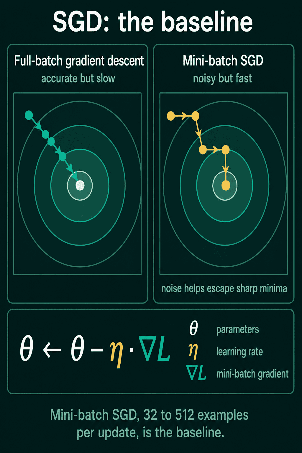
Batch gradient descent (also called full-batch) computes the gradient on the entire training set and makes one update per epoch. The gradient is exact for that data, so the path is smooth, but one update needs a full pass over the data, and millions of examples may not fit in memory at once.
Stochastic gradient descent in its original sense uses one example per update. Updates are cheap and frequent, but a gradient computed from one example can point quite far from the full-data gradient, so the path jumps around.
Mini-batch gradient descent averages the gradient over a small random batch. It gets many updates per epoch, each one far less noisy than a single-example update. When people say "SGD" in deep learning, they usually mean this version, and torch.optim.SGD applies the update to whatever batch the loop gives it.
The code below trains the same linear regression model on 1,024 synthetic examples for 5 epochs with each of the three batch sizes and the same learning rate, then reports the loss on the full dataset:
1import torch
2from torch.utils.data import TensorDataset, DataLoader
3
4torch.manual_seed(0)
5X = torch.randn(1024, 10)
6true_w = torch.randn(10, 1)
7y = X @ true_w + 0.5 * torch.randn(1024, 1)
8dataset = TensorDataset(X, y)
9
10def train(batch_size, lr, epochs=5):
11    torch.manual_seed(0)
12    model = torch.nn.Linear(10, 1)
13    optimizer = torch.optim.SGD(model.parameters(), lr=lr)
14    loss_fn = torch.nn.MSELoss()
15    loader = DataLoader(dataset, batch_size=batch_size, shuffle=True)
16    steps = 0
17    for epoch in range(epochs):
18        for xb, yb in loader:
19            optimizer.zero_grad()
20            loss = loss_fn(model(xb), yb)
21            loss.backward()
22            optimizer.step()
23            steps += 1
24    with torch.no_grad():
25        full_loss = loss_fn(model(X), y).item()
26    return steps, full_loss
27
28for name, bs in [("full batch", 1024), ("stochastic", 1), ("mini-batch", 32)]:
29    steps, loss = train(bs, lr=0.01)
30 print(f"{name:>10} batch_size={bs:<5} updates={steps:<5} loss={loss:.3f}")1full batch batch_size=1024 updates=5 loss=12.838
2stochastic batch_size=1 updates=5120 loss=0.311
3mini-batch batch_size=32 updates=160 loss=0.272With the same five passes over the data, full batch made 5 updates and is still far from a good fit at a loss of 12.838. Stochastic made 5,120 updates and got close, but each one processed a single example, which uses little of the hardware's parallelism. Mini-batch reached the lowest loss, 0.272, with 160 updates of 32 examples each. The noise in the target is 0.5, so a perfect fit would sit near a loss of 0.25.
How batch size changes gradient noise
A mini-batch gradient is an estimate of the full-data gradient, and a bigger batch gives a closer estimate. The next snippet measures how close. It samples 200 random batches of each size and records the average distance between the batch gradient and the full-data gradient for the model's weights:
1import torch
2
3torch.manual_seed(0)
4X = torch.randn(1024, 10)
5true_w = torch.randn(10, 1)
6y = X @ true_w + 0.5 * torch.randn(1024, 1)
7
8model = torch.nn.Linear(10, 1)
9loss_fn = torch.nn.MSELoss()
10
11def weight_grad(idx):
12    model.zero_grad()
13    loss_fn(model(X[idx]), y[idx]).backward()
14    return model.weight.grad.clone()
15
16full_grad = weight_grad(torch.arange(1024))
17for bs in [1, 8, 32, 128, 512]:
18    errors = []
19    for _ in range(200):
20        idx = torch.randperm(1024)[:bs]
21        errors.append((weight_grad(idx) - full_grad).norm())
22    print(f"batch_size={bs:<4} avg distance from full gradient={torch.stack(errors).mean():.3f}")
23print(f"size of the full gradient itself: {full_grad.norm():.3f}")1batch_size=1 avg distance from full gradient=21.383
2batch_size=8 avg distance from full gradient=8.312
3batch_size=32 avg distance from full gradient=4.401
4batch_size=128 avg distance from full gradient=1.995
5batch_size=512 avg distance from full gradient=0.755
6size of the full gradient itself: 7.611A single example's gradient is off by 21.383, almost three times the size of the true gradient (7.611). Going from 32 to 128 examples, four times the compute per step, cut the error from 4.401 to 1.995, under half its size. That is the main trade-off: the cost of a step grows in proportion to the batch, and the gradient's accuracy grows much more slowly, roughly with the square root of the batch.
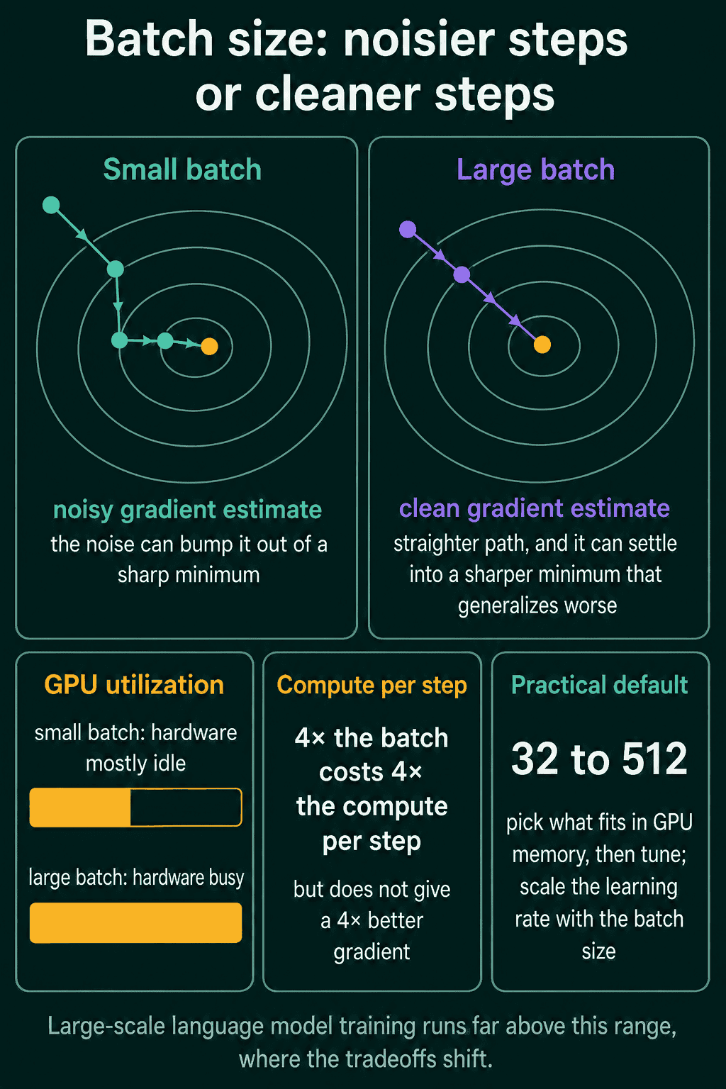
Some of that noise is useful. A sharp minimum is a low point of the loss where the loss climbs steeply as soon as the parameters move a little, and models that settle in one often do worse on data they were not trained on. A noisy gradient pushes the parameters around from step to step, which can knock them out of a sharp minimum or off a saddle point, a spot where the gradient is near zero but the loss still falls in some direction. Very large batches remove most of that noise, and large-batch training can settle into sharper minima that generalize worse.
How batch size interacts with the learning rate
A cleaner gradient can support a larger step, and a larger batch means fewer updates per epoch, so with the same learning rate, training covers less ground per epoch. The common fix is the linear scaling rule: when the batch size is multiplied by $k$, multiply the learning rate by $k$ too. This reuses train from the first snippet:
1for bs, lr in [(32, 0.01), (256, 0.01), (256, 0.08)]:
2    steps, loss = train(bs, lr=lr)
3 print(f"batch_size={bs:<4} lr={lr:<5} updates={steps:<4} loss={loss:.3f}")1batch_size=32 lr=0.01 updates=160 loss=0.272
2batch_size=256 lr=0.01 updates=20 loss=6.967
3batch_size=256 lr=0.08 updates=20 loss=0.264Raising the batch from 32 to 256 with the learning rate unchanged left the loss at 6.967 after 5 epochs. Scaling the learning rate by the same factor of 8, to 0.08, brought it to 0.264 with the same 20 updates. The rule is a starting point rather than a law, and at very large batch sizes it is usually combined with a warmup period of small learning rates at the start. The learning rate post covers how to find a working value.
How to choose a batch size
- GPU utilization. A GPU processes the examples in a batch in parallel, so a batch of 8 leaves most of it idle, and a batch of 256 can take close to the same wall-clock time per step. Larger batches often finish an epoch faster even though each step does more arithmetic.
- Memory. Activations for every example in the batch are kept for backpropagation, so memory grows with the batch size. The largest batch that fits sets an upper limit.
- A starting range. 32 to 512 works for most tasks. Pick a size in that range that fits in memory, often a power of two such as 64 or 128, and tune from there. Large language model training runs far above this range, with batches measured in millions of tokens, and the trade-offs shift at that scale.
If training becomes unstable after raising the batch size and the learning rate together, lower the learning rate first. If the loss improves more slowly after only raising the batch size, raise the learning rate.
Common mistakes
- Changing the batch size without touching the learning rate. In the run above, a batch 8 times larger with the same learning rate left the loss at 6.967 instead of 0.272.
- Comparing runs by epoch count alone. Batch size 32 and batch size 256 make different numbers of updates per epoch, so compare the number of updates and wall-clock time as well.
- Forgetting
shuffle=Trueon the trainingDataLoader. Without it, every epoch feeds the batches in the same order, and if the data is sorted by label, batches can hold a single class and the gradients swing between classes. - Summing the loss instead of averaging it. A summed loss grows with the batch size, and so does its gradient, which changes the effective learning rate each time the batch size changes.
Related concepts
Momentum keeps a running average of past gradients, which smooths out some of the mini-batch noise. Adam and AdamW scale each parameter's step by a running estimate of its gradient size and train on the same mini-batches, and the optimizers post covers both. Gradient accumulation adds up gradients over several small batches before calling optimizer.step(), which gives the gradient of a larger batch when that batch does not fit in memory.
QuiddityML teaches SGD and batch size effects as two concepts in the ML Foundation track, and the exercises include writing the SGD update step from its equation, spotting the plus sign that turns it into gradient ascent, and working out what happens to training when the batch size doubles and the learning rate stays fixed.