30 September 2026 · 12 min read
Learning rate schedules explained: warmup, cosine annealing, step decay, and ReduceLROnPlateau
A learning rate schedule changes the step size of training as the run goes on, usually large at the start and small at the end. This post explains why a fixed learning rate falls short, how linear warmup, cosine annealing, step decay, and ReduceLROnPlateau work, and how to set each one up in PyTorch.
A learning rate schedule is a rule that changes the learning rate while a model trains, instead of keeping it at one value for the whole run. The usual pattern is a large rate early, when the model is far from a good solution, and a small rate late, when it is close to one. Many training scripts use a schedule, and picking the wrong one, or wiring it up wrong, can leave a model at a higher loss than the same code with a better schedule.
What the learning rate does
Training updates a model's parameters $\theta$ over and over. On each step it computes the gradient $\nabla L(\theta)$, the direction in which the loss $L$ grows fastest, and moves the parameters a small distance the other way:
$$\theta \leftarrow \theta - \eta , \nabla L(\theta)$$
The learning rate $\eta$ sets how far each step goes. A gradient of 2.0 with $\eta = 0.1$ moves a parameter by 0.2. How to pick a starting value is covered in what a learning rate is and how to pick one. A schedule starts from that value and changes it as training goes on, so $\eta$ becomes $\eta_t$, the learning rate at step $t$.
Why a fixed learning rate is a compromise
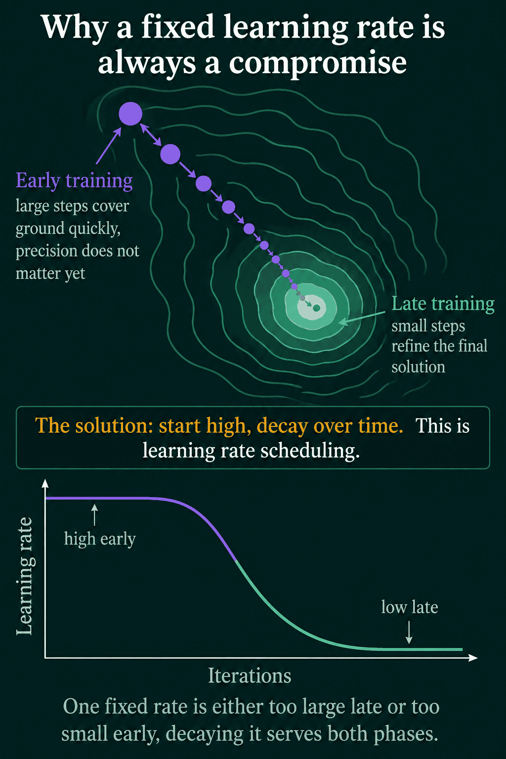
Training has two phases that want different step sizes.
- Early in training the parameters are far from a good solution. Large steps cover the distance quickly, and small errors in direction do little harm because the next step corrects them.
- Late in training the parameters are close to a low point of the loss. A large step jumps past the low point and lands on the other side, so the loss bounces around a value above the minimum instead of settling into it.
A single fixed value has to pick one of these. A large rate makes fast early progress and then bounces at the end. A small rate settles well at the end but spends most of the run creeping forward. Starting high and lowering the rate over time gets the fast start and the precise finish in the same run, which is what learning rate scheduling is.
How a scheduler works in PyTorch
In PyTorch the learning rate lives in the optimizer, in optimizer.param_groups[0]["lr"]. A scheduler is an object that wraps the optimizer and rewrites that value each time scheduler.step() is called. Depending on the schedule, scheduler.step() is called once per batch or once per epoch (one full pass over the training data), and the schedule's lengths, such as T_max or step_size, count those calls.
Linear warmup
The first steps of training are the least stable. The weights are random, so the gradients they produce are large and point in inconsistent directions. Adaptive optimizers such as Adam add a second problem: Adam divides each parameter's step by the square root of $\hat{v}$, a running average of that parameter's squared gradients. At step 5, $\hat{v}$ has been estimated from five gradients, so it is noisy, and dividing by a noisy number gives erratic step sizes. A full-sized learning rate on top of that can push the weights into a bad region early in the run, and the run may not recover from it.
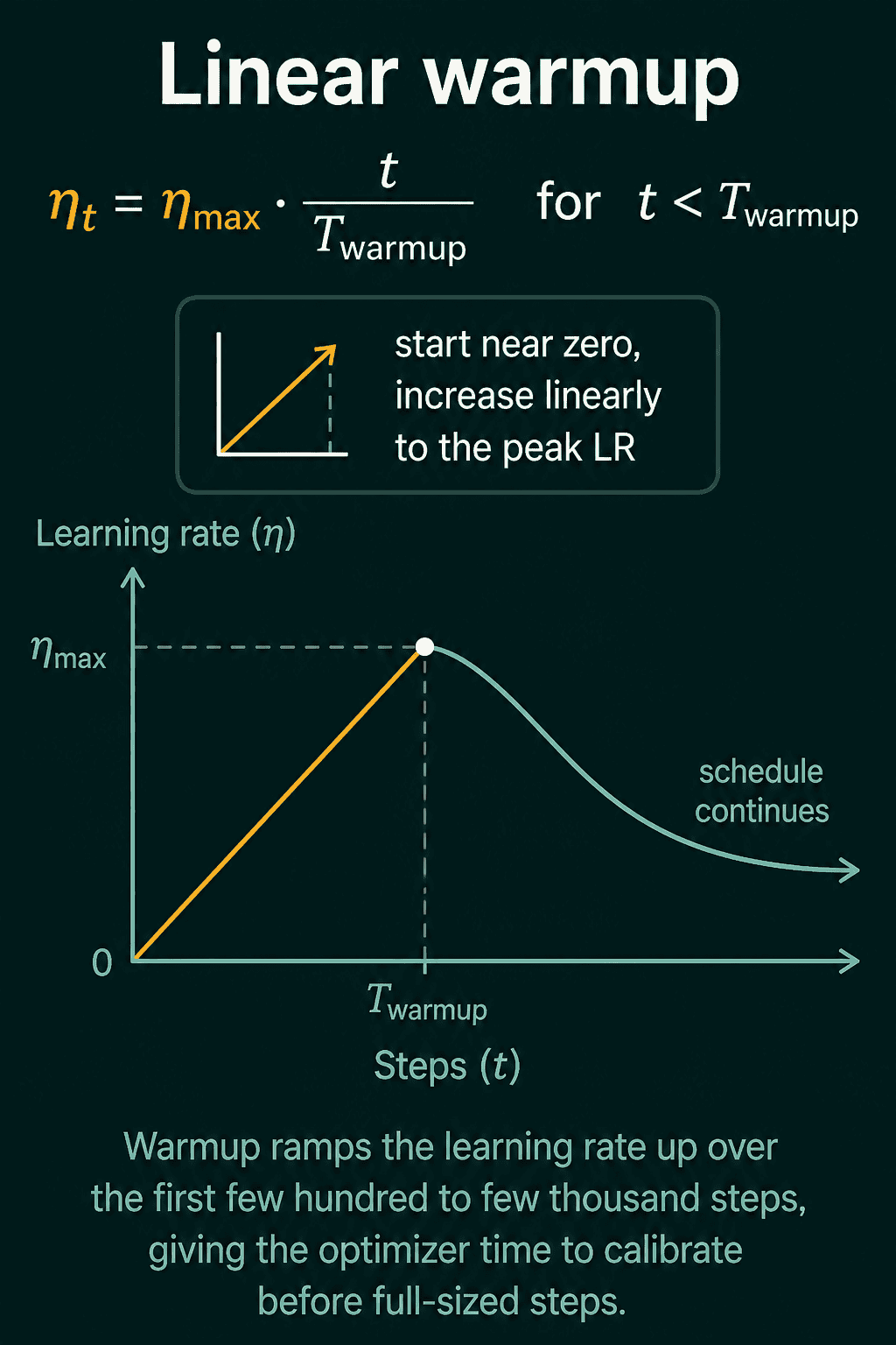
Linear warmup starts the learning rate near zero and raises it in a straight line to its peak value $\eta_{\max}$ over the first $T_{\text{warmup}}$ steps:
$$\eta_t = \eta_{\max} \cdot \frac{t}{T_{\text{warmup}}} \quad \text{for } t < T_{\text{warmup}}$$
At $t = 0$ the rate is 0, halfway through warmup it is $\eta_{\max}/2$, and at $t = T_{\text{warmup}}$ it reaches the peak. By then the gradients are less erratic and Adam's $\hat{v}$ has been averaged over hundreds of steps. Warmup lengths from a few hundred to a few thousand steps are common. Large models and large batch sizes tend to need it most, since one bad early update can undo a good initialization.
Cosine annealing
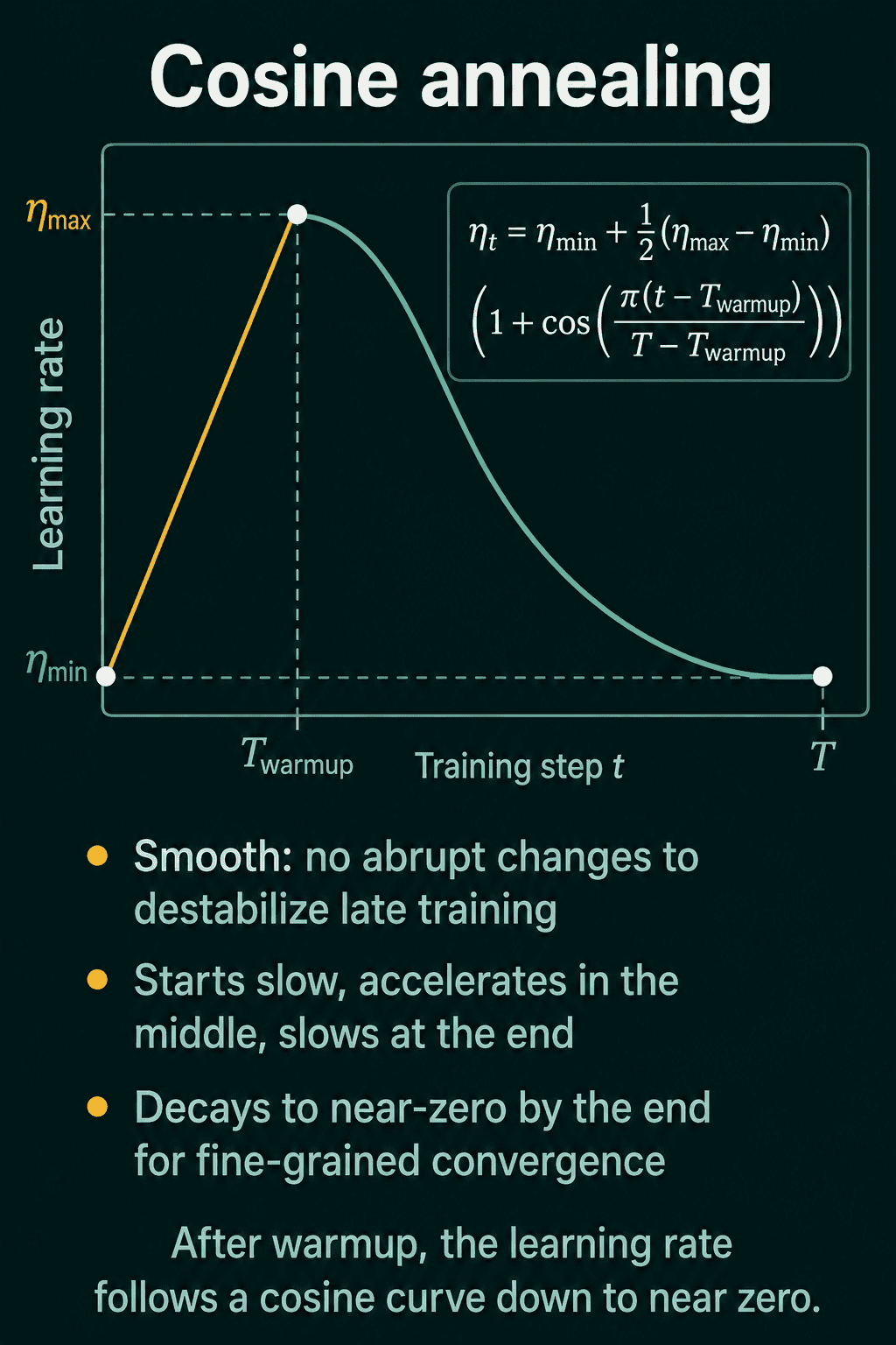
After warmup, the learning rate needs to come down. Cosine annealing lowers it along half of a cosine curve, from the peak $\eta_{\max}$ to a floor $\eta_{\min}$ at the last step $T$:
$$\eta_t = \eta_{\min} + \frac{1}{2}(\eta_{\max} - \eta_{\min})\left(1 + \cos\left(\pi \cdot \frac{t - T_{\text{warmup}}}{T - T_{\text{warmup}}}\right)\right)$$
The fraction inside the cosine is how far through the decay phase the run is, going from 0 right after warmup to 1 at the end. Over that range $\cos$ goes from 1 to -1, so the factor $\frac{1}{2}(1 + \cos)$ goes from 1 to 0 and the rate moves from $\eta_{\max}$ down to $\eta_{\min}$. The curve is flat at both ends and steepest in the middle: the rate stays near the peak for a while after warmup, drops fastest halfway through, and eases into the floor at the end. There are no sudden jumps, and the final steps run at a rate close to $\eta_{\min}$, which is where the precise settling happens.
The two formulas together fit in one short function:
1import math
2
3def get_lr(step, peak_lr, warmup_steps, total_steps, min_lr=1e-6):
4    """Linear warmup to peak_lr, then cosine decay to min_lr."""
5    if step < warmup_steps:
6        return peak_lr * step / warmup_steps
7    progress = (step - warmup_steps) / (total_steps - warmup_steps)
8    return min_lr + 0.5 * (peak_lr - min_lr) * (1 + math.cos(math.pi * progress))
9
10for step in [0, 50, 100, 325, 550, 775, 1000]:
11 print(f"step {step:4d} lr {get_lr(step, 1e-3, 100, 1000):.2e}")1step 0 lr 0.00e+00
2step 50 lr 5.00e-04
3step 100 lr 1.00e-03
4step 325 lr 8.54e-04
5step 550 lr 5.01e-04
6step 775 lr 1.47e-04
7step 1000 lr 1.00e-06With a peak of 1e-3, 100 warmup steps, and 1,000 steps in total, the rate is half the peak at step 50, reaches the peak at step 100, is back to half the peak at step 550 (the middle of the decay phase), and ends at the floor of 1e-6.
Warmup and cosine in PyTorch
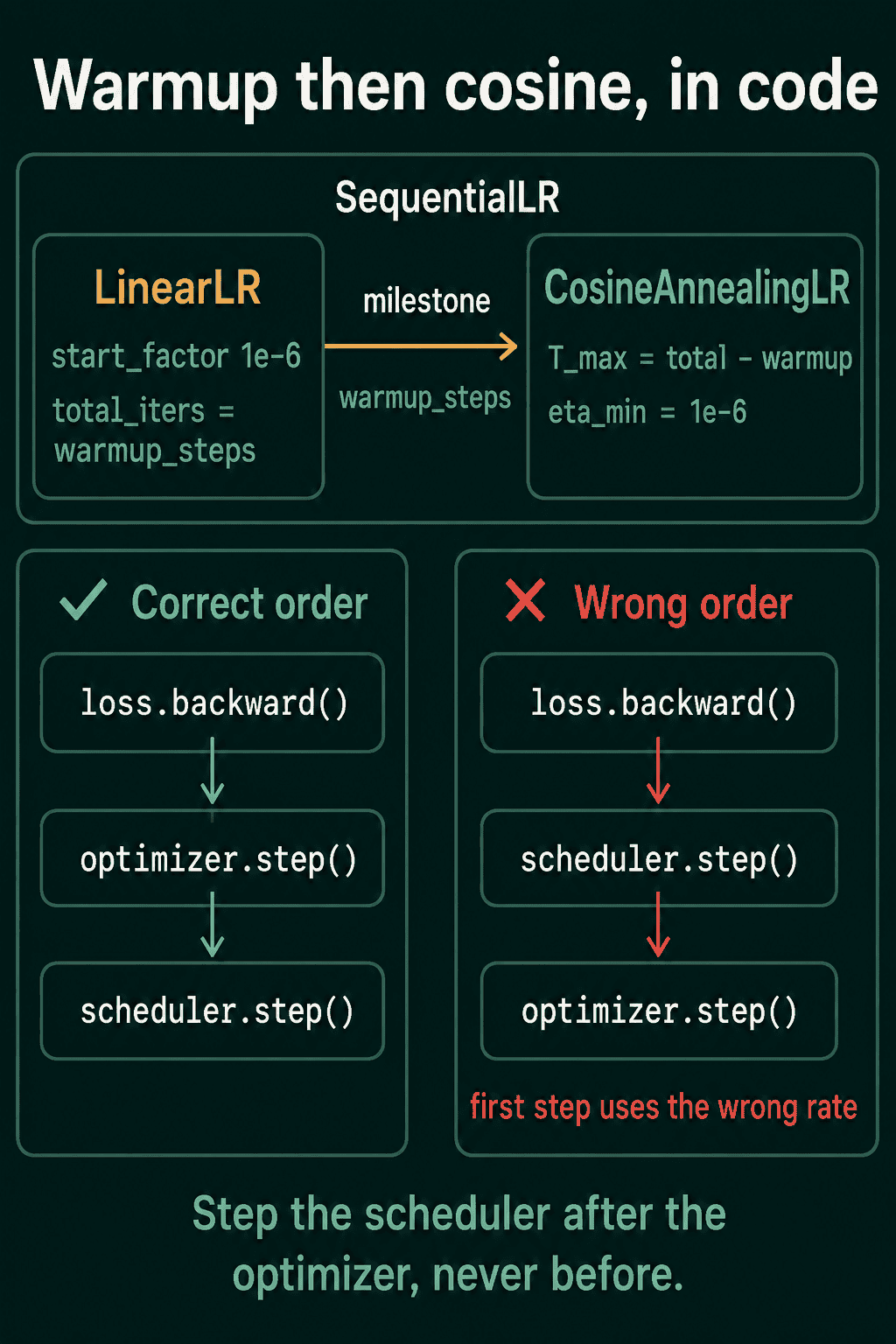
PyTorch builds the same schedule from three pieces. LinearLR multiplies the base learning rate by a factor that moves from start_factor to end_factor over total_iters steps, which gives the warmup. CosineAnnealingLR does the cosine decay over T_max steps down to eta_min. SequentialLR runs the first scheduler until the step count reaches the milestones value, then hands over to the second.
1import torch
2from torch.optim.lr_scheduler import LinearLR, CosineAnnealingLR, SequentialLR
3
4model = torch.nn.Linear(10, 1)
5optimizer = torch.optim.AdamW(model.parameters(), lr=1e-3)
6
7warmup_steps, total_steps = 100, 1000
8warmup = LinearLR(optimizer, start_factor=1e-6, end_factor=1.0, total_iters=warmup_steps)
9cosine = CosineAnnealingLR(optimizer, T_max=total_steps - warmup_steps, eta_min=1e-6)
10scheduler = SequentialLR(optimizer, schedulers=[warmup, cosine], milestones=[warmup_steps])
11
12X, y = torch.randn(256, 10), torch.randn(256, 1)
13for step in range(total_steps):
14    lr = optimizer.param_groups[0]["lr"]
15    if step in (0, 50, 100, 325, 550, 775, 999):
16        print(f"step {step:4d}  lr {lr:.2e}")
17    loss = torch.nn.functional.mse_loss(model(X), y)
18    optimizer.zero_grad()
19    loss.backward()
20    optimizer.step()
21 scheduler.step()1step 0 lr 1.00e-09
2step 50 lr 5.00e-04
3step 100 lr 1.00e-03
4step 325 lr 8.54e-04
5step 550 lr 5.00e-04
6step 775 lr 1.47e-04
7step 999 lr 1.00e-06The printed rates agree with get_lr to two significant figures, and the last line is step 999 because the loop runs steps 0 to 999. The one visible difference is step 0, where LinearLR starts at start_factor times the base rate, 1e-9, instead of exactly 0. T_max is total_steps - warmup_steps because the cosine part only runs after warmup ends.
scheduler.step() goes after optimizer.step(). If the order is reversed, PyTorch prints a warning and skips the first value of the schedule, so each optimizer step runs one step ahead of the schedule and the first step uses the wrong rate.
Step decay
Step decay is an older and simpler schedule: keep the rate fixed, and multiply it by a factor $\gamma$ (gamma, a number below 1) every $T_{\text{step}}$ epochs. Starting from $\eta_0$:
$$\eta_t = \eta_0 \cdot \gamma^{\lfloor t / T_{\text{step}} \rfloor}$$
$\lfloor t / T_{\text{step}} \rfloor$ rounds down, so it counts how many full blocks of $T_{\text{step}}$ epochs have passed, and each block multiplies the rate by $\gamma$ once more. A common setting for image classifiers trained with SGD was $\eta_0 = 0.1$ and $\gamma = 0.1$ every 30 epochs. StepLR implements it and is stepped once per epoch:
1import torch
2
3model = torch.nn.Linear(10, 1)
4optimizer = torch.optim.SGD(model.parameters(), lr=0.1, momentum=0.9)
5scheduler = torch.optim.lr_scheduler.StepLR(optimizer, step_size=30, gamma=0.1)
6
7for epoch in range(100):
8    if epoch in (0, 29, 30, 59, 60, 90):
9        print(f"epoch {epoch:3d}  lr {optimizer.param_groups[0]['lr']:.0e}")
10    # ... one epoch of training batches, each ending in optimizer.step() ...
11    optimizer.step()
12 scheduler.step()1epoch 0 lr 1e-01
2epoch 29 lr 1e-01
3epoch 30 lr 1e-02
4epoch 59 lr 1e-02
5epoch 60 lr 1e-03
6epoch 90 lr 1e-04The rate holds at 0.1 through epoch 29, then drops by 10 times at epochs 30, 60, and 90. The loss usually falls sharply right after each drop and then flattens until the next one. The drawback is that the drop epochs are extra settings to choose by hand, and they have to be chosen again when the length of the run changes. Cosine annealing needs only the total length, which is one reason it has replaced step decay in many newer training setups. When exact step points are needed, MultiStepLR takes a list of epochs such as milestones=[30, 60, 90].
ReduceLROnPlateau
Cosine annealing and step decay both need to know in advance how long training will run. ReduceLROnPlateau does not. It watches a metric measured on a validation set, a slice of data held back from training so the metric says how the model does on examples it has not fit, and cuts the learning rate when that metric stops improving. Its main settings:
mode:"min"when lower is better (a loss),"max"when higher is better (accuracy).factor: what to multiply the rate by on each cut.patience: how many epochs without improvement to allow. The cut happens when the count of such epochs goes abovepatience.min_lr: a floor the rate will not go below.
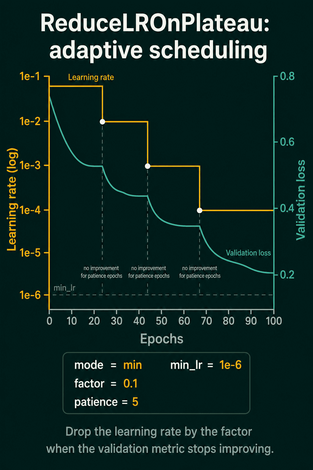
Unlike the other schedulers, its step() takes the metric as an argument:
1import torch
2
3model = torch.nn.Linear(10, 1)
4optimizer = torch.optim.SGD(model.parameters(), lr=0.1)
5scheduler = torch.optim.lr_scheduler.ReduceLROnPlateau(
6    optimizer, mode="min", factor=0.1, patience=2, min_lr=1e-6
7)
8
9val_losses = [0.90, 0.70, 0.60, 0.61, 0.60, 0.62, 0.63, 0.50, 0.49, 0.49, 0.50, 0.50]
10for epoch, val_loss in enumerate(val_losses):
11    optimizer.step()  # stands in for one epoch of training
12    scheduler.step(val_loss)
13 print(f"epoch {epoch:2d} val_loss {val_loss:.2f} lr {optimizer.param_groups[0]['lr']:.0e}")1epoch 0 val_loss 0.90 lr 1e-01
2epoch 1 val_loss 0.70 lr 1e-01
3epoch 2 val_loss 0.60 lr 1e-01
4epoch 3 val_loss 0.61 lr 1e-01
5epoch 4 val_loss 0.60 lr 1e-01
6epoch 5 val_loss 0.62 lr 1e-02
7epoch 6 val_loss 0.63 lr 1e-02
8epoch 7 val_loss 0.50 lr 1e-02
9epoch 8 val_loss 0.49 lr 1e-02
10epoch 9 val_loss 0.49 lr 1e-02
11epoch 10 val_loss 0.50 lr 1e-02
12epoch 11 val_loss 0.50 lr 1e-03The lowest loss so far is 0.60 at epoch 2. Epochs 3, 4, and 5 do not beat it (matching 0.60 at epoch 4 does not count as an improvement), so after epoch 5 the count is 3, which is above patience=2, and the rate drops to 0.01. The count resets after the cut. Epochs 7 and 8 set new bests, then epochs 9, 10, and 11 fail to beat 0.49, and the rate drops again to 0.001.
ReduceLROnPlateau has no warmup built in, and it needs a validation pass at regular intervals, which costs extra compute on large runs. It is a common choice for smaller models and for runs whose length is not known ahead of time.
Does a schedule change the result?
The experiment below trains a linear model on 2,000 noisy examples with plain SGD, a batch of 16 random rows per step, and a starting rate of 0.05 for 2,000 steps. It compares a constant rate, step decay (divide by 10 every 600 steps), and cosine annealing, and measures the final loss on the full dataset. The last line is the lowest loss a linear model can reach on this data, solved directly with least squares.
1import torch
2
3torch.manual_seed(0)
4X = torch.randn(2000, 20)
5y = X @ torch.randn(20, 1) + 0.5 * torch.randn(2000, 1)
6
7def train(schedule, steps=2000, lr=0.05):
8    torch.manual_seed(1)
9    model = torch.nn.Linear(20, 1)
10    optimizer = torch.optim.SGD(model.parameters(), lr=lr)
11    scheduler = None
12    if schedule == "step":
13        scheduler = torch.optim.lr_scheduler.StepLR(optimizer, step_size=600, gamma=0.1)
14    elif schedule == "cosine":
15        scheduler = torch.optim.lr_scheduler.CosineAnnealingLR(optimizer, T_max=steps)
16    for _ in range(steps):
17        idx = torch.randint(0, 2000, (16,))  # a mini-batch of 16 random rows
18        loss = torch.nn.functional.mse_loss(model(X[idx]), y[idx])
19        optimizer.zero_grad()
20        loss.backward()
21        optimizer.step()
22        if scheduler is not None:
23            scheduler.step()
24    with torch.no_grad():
25        return torch.nn.functional.mse_loss(model(X), y).item()
26
27for schedule in ["constant", "step", "cosine"]:
28    print(f"{schedule:8s}  final loss {train(schedule):.4f}")
29
30# The lowest loss a linear model can reach on this data, solved directly
31Xb = torch.cat([X, torch.ones(2000, 1)], dim=1)
32w = torch.linalg.lstsq(Xb, y).solution
33print(f"least squares {torch.nn.functional.mse_loss(Xb @ w, y).item():.4f}")1constant final loss 0.2567
2step final loss 0.2346
3cosine final loss 0.2348
4least squares 0.2343With a constant rate the model ends 0.0224 above the least-squares loss, because each noisy mini-batch step at 0.05 keeps moving the weights around the minimum. Step decay and cosine annealing both end within 0.0005 of it, since their last few hundred steps run at a rate small enough to settle. On this problem the two decaying schedules finish in the same place. The practical difference between them is that step decay needed a drop point (600 steps) chosen by hand, and cosine annealing needed only the total number of steps.
Which schedule to use
| Schedule | Needs total length | Reacts to validation | Common use |
|---|---|---|---|
| Warmup + cosine | yes | no | transformers, most large runs |
| Step decay | yes, to place drops | no | older SGD image recipes |
| ReduceLROnPlateau | no | yes | small models, open-ended runs |
| Constant | no | no | quick experiments, debugging |
- Default to warmup plus cosine when the number of training steps is known, especially with Adam or AdamW. Warmup at 1 to 10 percent of the total steps and a floor near zero are reasonable starting points.
- Use ReduceLROnPlateau when the length of the run is open-ended and a validation metric is cheap to compute.
- Keep a constant rate while debugging. A schedule adds one more thing that can hide a bug, so it is easier to add it once the model trains at a fixed rate.
- Retune the peak rate after adding warmup. Warmup often lets a run tolerate a higher peak than the same run without it.
Common mistakes
- Stepping the scheduler before the optimizer. PyTorch skips the first value of the schedule, and each step then uses the rate meant for the next one.
- Mixing per-batch and per-epoch steps.
T_maxandstep_sizecount calls toscheduler.step(). SettingT_maxto the number of epochs and then callingscheduler.step()once per batch finishes the whole decay in the first few epochs. - Running past
T_max. PyTorch'sCosineAnnealingLRdoes not stop at the floor. It follows the cosine back up, so with a base rate of 0.1 andT_max=10the rate is 0 at step 10 and back at 0.1 at step 20. - Calling
ReduceLROnPlateau.step()with no argument, or with the training loss. It needs the validation metric to decide anything, and the training loss usually keeps falling after the validation loss has stopped improving. - Forgetting that a scheduler overrides the optimizer's rate. Changing
optimizer.param_groups[0]["lr"]by hand while a scheduler is running gets overwritten or compounded at the nextscheduler.step().
Related concepts
The learning rate post covers picking the starting value that a schedule then shapes. Adam and the other optimizers decide the direction and per-parameter size of each step, and a schedule scales all of those steps together, which is why warmup and Adam are usually used as a pair. Early stopping is the close relative of ReduceLROnPlateau: both watch the validation metric, and one lowers the rate when it stalls while the other ends training. The training loop is where scheduler.step() sits, right after optimizer.step().
QuiddityML teaches each of these schedules as its own concept in the ML Foundation track, and the exercises include writing get_lr for warmup plus cosine from the formula, ordering the lines that set up SequentialLR, and tracing a ReduceLROnPlateau run epoch by epoch to find where the rate drops (quiddityml.com).